This is a test case notebook which demonstrates how EMA background subtraction works. After going through this the user should be familiar with the method and how the parameter selection and scene affect the outcome. The source code can be found here. This code was written for a raspberry pi zero, so while neural nets and other ML models will for sure out perform this, this can be used on a very low powered device and needs no training, just some intuitive parameter selection.
Initialisation and false detections
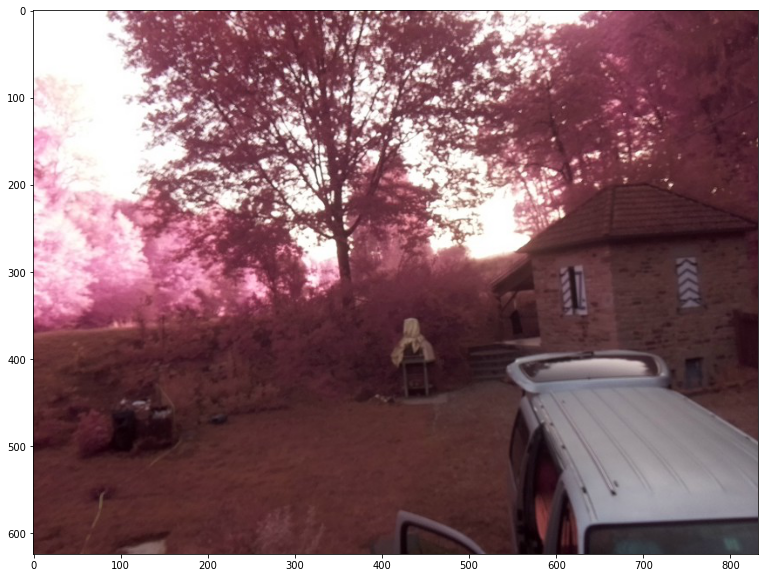
My experience so far is that false detections are a greater issue than tuning the system for true detections and tuning the system can be very painful as the system needs time to learn the background, so changing settings often means true results come minutes later. To speed this up good initialisation of the detector class is required. To simulate a noisy camera, we add noise to the image at each update, to show how a good initialisation can improve results we create two detectors one initialised with the perfect values the other with zeros. We can then quantify the convergence of the false detections and the variance.
from motion_detectors import EMAV_background_subtracting_motion_detection as bgd
#%matplotlib widget
from PIL import Image
import numpy as np
from scipy.ndimage import zoom
import matplotlib.pyplot as plt
plt.rcParams['figure.figsize'] = [20, 10]
example = np.array(Image.open('example.jpg'))
variance = 100 # the variance to be used for simulated camera noise.

detector_no_initialisation = bgd(0.05,16,example.shape, initial_average=np.zeros(example.shape), initial_variance=1, minimum_variance=18)

detector_good_initialisation = bgd(0.05,16,example.shape, initial_average=example, initial_variance=variance, minimum_variance=18)
plt.imshow(example)
<matplotlib.image.AxesImage at 0x7fab89447d68>
false_postives_no_init = []
measured_variance_no_init  = []

false_postives_good_init = []
measured_variance_good_init  = []

for i in range(250):
    noisy_image = example+np.random.normal(0, variance**0.5, example.shape)
    # rember the camera clips values
    noisy_image[noisy_image<0]=0
    noisy_image[noisy_image>255]=255

    detections_no_init=detector_no_initialisation.apply(noisy_image)
    false_postives_no_init.append(np.sum(detections_no_init))
    measured_variance_no_init.append(np.mean(detector_no_initialisation.variance_background))

    detections_good_init=detector_good_initialisation.apply(noisy_image)
    false_postives_good_init.append(np.sum(detections_good_init))
    measured_variance_good_init.append(np.mean(detector_good_initialisation.variance_background))
    #plt.imshow(a,interpolation='nearest')

fig, ax = plt.subplots(1, 2)
ax[0].plot(false_postives_no_init)
ax[0].plot(false_postives_good_init)
ax[0].set_title('False Detections')
ax[0].set_xlabel('Iterations [-]')
ax[0].set_ylabel('False Detections [pixels]')
ax[1].plot(measured_variance_no_init)
ax[1].plot(measured_variance_good_init)
ax[1].set_title('Measured Variance')
ax[1].set_xlabel('Iterations [-]')
ax[1].set_ylabel('Variance [-]')
ax[1].set_yscale('log')
ax[1].legend(['No initilisation','Good initlisation'])
<matplotlib.legend.Legend at 0x7fab885126a0>
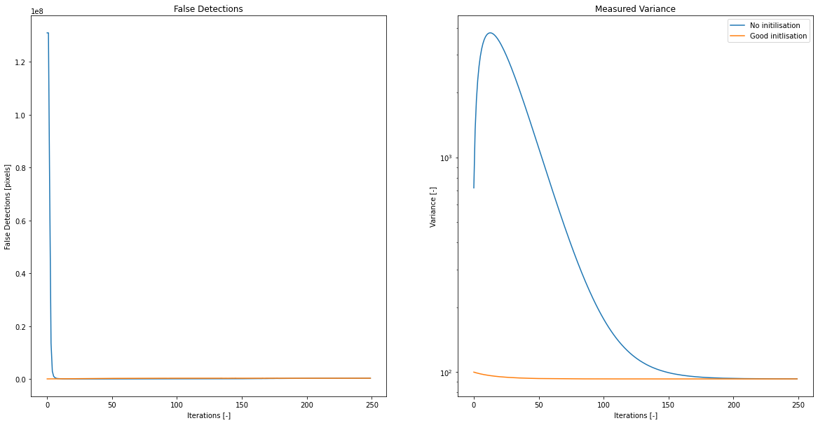
This might not seem like much but on a system like a rasperry pi zero an update can take 3 seconds, so the camera is essentially blind for the first 5 minutes after starting if the Variance is so poorly measured.
Motion detection
Now we have an initialised system how well can we detect motion which is not part of the background. The first test is to add a synthetic person to the images at random spaces and times. Here a copyright free image of a person is loaded and then a function got adding it to the image is defined.
person = zoom(np.array(Image.open('walking_man.jpg'))[:,:,0],0.3)<220
Now let’s add him to the image.
y=200
x=400

def insert_person(image,x,y,value=[35,120,120]):
    im=np.copy(image)
    sub = np.copy(im[x:x+person.shape[0],y:y+person.shape[1]])
    sub[person]=value

    im[x:x+person.shape[0],y:y+person.shape[1]]=sub
    return im

image = insert_person(example,400,200)
truth = insert_person(np.zeros(example.shape[:-1],dtype=bool),400,200,1)
plt.figure()
plt.imshow(image,interpolation='nearest')
plt.figure()
plt.imshow(truth,interpolation='nearest')
<matplotlib.image.AxesImage at 0x7fab8777f518>

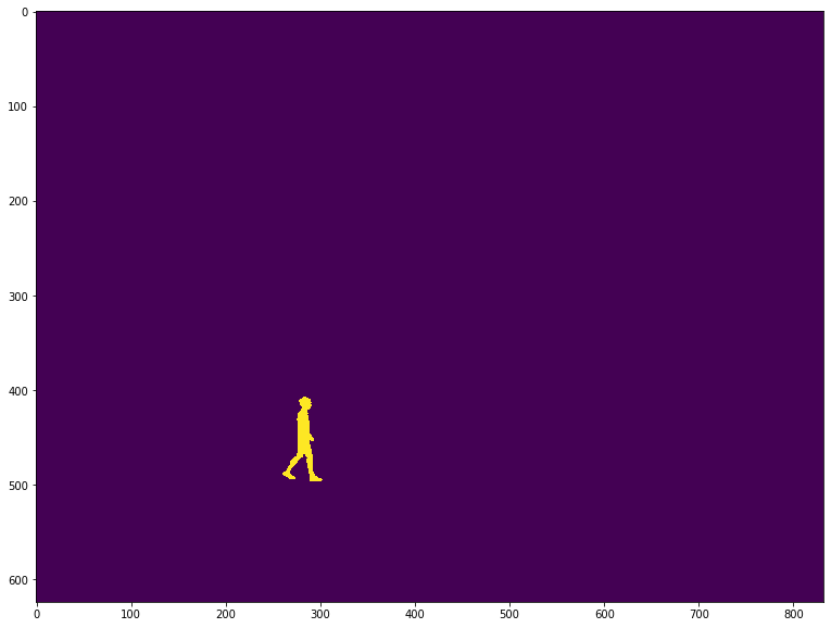
Now a little green man is walking across the grass. We can test detection for various weights and see if we can recover visually the person.
weights = [0.01, 0.05, 0.1, 0.5, 0.9]
detectors={w:bgd(w,9,example.shape, initial_average=example, initial_variance=variance) for w in weights}
background_counts={}
training_iterations = 50
#train the background
for i in range(training_iterations):
    noisy_image = example+np.random.normal(0, variance**0.5, example.shape)
    # remember the camera clips values
    noisy_image[noisy_image<0]=0
    noisy_image[noisy_image>255]=255
    noisy_image=noisy_image.astype(np.uint8)
    for w,detector in detectors.items():
        det = detector.apply(noisy_image)
        if background_counts.get(w,None) is None:
            background_counts[w]=np.sum(det)/training_iterations
        else:
            background_counts[w]+=np.sum(det)/training_iterations

#apply the image with person
masks = {w:d.apply(image) for w,d in detectors.items()}
rows=2
fig, ax = plt.subplots(rows,1+ len(weights)//rows)
x=0
y=0
for i,t in enumerate(masks.items()):
    if i==1+len(masks)//rows:
        x=0
        y+=1
    w=t[0]
    m=t[1]
    ax[y,x].imshow(m)
    ax[y,x].set_title('weight = '+str(w))
    x+=1
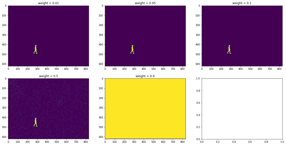
Clearly the higher weight values have less memory of the scene and it’s variance, this leads to noise being detected as a movements. The question is what happens is the person stays there for each detector?
size_of_person = np.sum(person)

#counts = {w:[(np.sum(masks[w])-background_counts[w])] for w in weights}
#counts = {w:[(np.sum(masks[w]))] for w in weights}
counts = {w:[] for w in weights}
for i in range(120):
    noisy_image = image+np.random.normal(0, variance**0.5, example.shape)
    # rember the camera clips values
    noisy_image[noisy_image<0]=0
    noisy_image[noisy_image>255]=255
    for w,detector in detectors.items():
        counts[w].append(np.sum(np.logical_and(detector.apply(noisy_image),truth)))
plt.figure()
for w,c in counts.items():
    plt.plot([x for x in c])
plt.legend([str(x) for x in counts], title='Training Weight')
plt.xlim([0,120])
(0.0, 120.0)
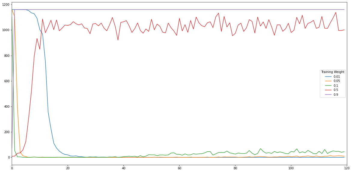
As one would expect the smaller the training weight the more iteration until the person is learnt as part of the background. There are essentially three behaviours which can be observered, the highest weights cannot differentiate between the person and noise, so they are constantly detecting pixels in this location. The low weights adapt quickly to the person, with the adaption being longer for smaller weights. The weight of 0.5 represents an intersting case, the average and variance have adapted quickly to the presence of the person, so it is initially not sensitive to the person, however after several itterartions the variance will decrease, and it is again sensitve to noise.
Moving background
To demonstrate both the utlitity of the variance tracking for motion segmentation, and the issues with false postives here is a section where a moving bakground is simulated. While this would be nicer with a video, I did not have the foresight to take one, also it would increase the repo size. Instead, motion is simulated using the swirl function, creating a region in the center of the image which is deformed.
from skimage.transform import swirl

series = [(255*swirl(example, rotation=0, strength=s, radius=700)).astype(np.uint8) for s in np.linspace(0,2,4) ]

rows=2
fig, ax = plt.subplots(rows, len(series)//rows)
x=0
y=0
for i,s in enumerate(series):
    if i==len(series)//rows:
        x=0
        y+=1
    ax[y,x].imshow(s)
    x+=1
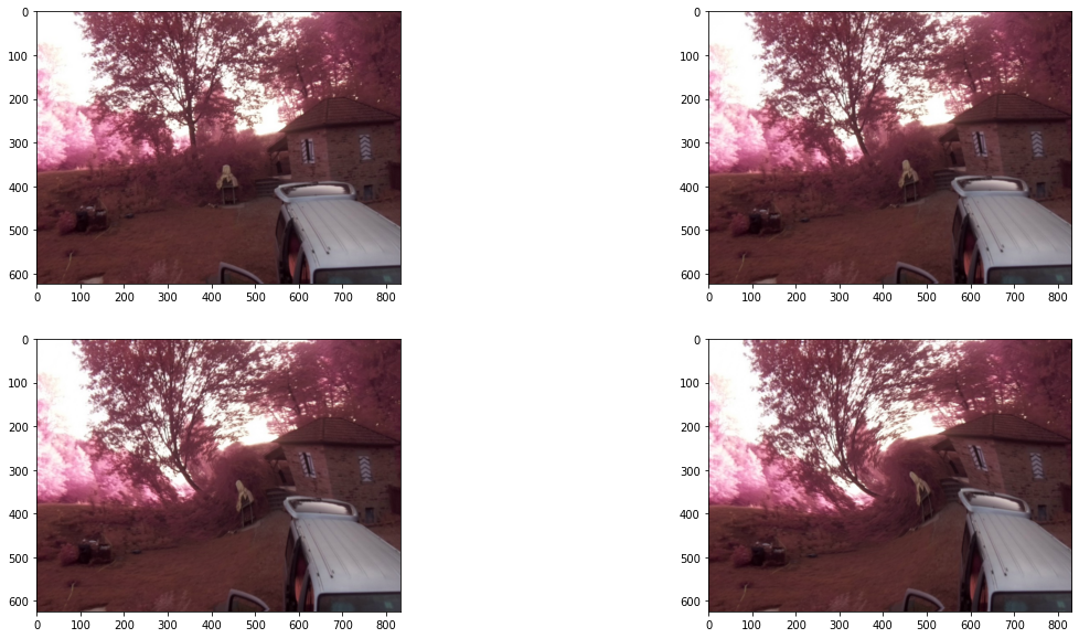
No to show how this influecne the learning we can run a series of detectors with different learning weights.
Ultimately only two things are of interest, what happens to the variance in the regions where the swirl is occuring? and how many times is this deformation classified as a moving object by each detector?
#Initalise the detectors and train to the static noisy background.

weights = [0.001, 0.01, 0.05, 0.25,0.5]
variance=100
detectors={w:bgd(w,10,example.shape, initial_average=example, initial_variance=variance, minimum_variance=0) for w in weights}
background_counts={}
training_iterations = 50
#train the background
for i in range(training_iterations):
    noisy_image = example + np.random.normal(0, variance**0.5, example.shape)
    # remember the camera clips values
    noisy_image[noisy_image<0]=0
    noisy_image[noisy_image>255]=255
    for w,detector in detectors.items():
        det = detector.apply(noisy_image)
        if background_counts.get(w,None) is None:
            background_counts[w]=np.sum(det)/training_iterations
        else:
            background_counts[w]+=np.sum(det)/training_iterations

init_vars = {w:np.copy(d.variance_background) for w,d in detectors.items()}
counts = {w:[] for w in weights}
var = {w:[] for w in weights}

for cycle in range(15):
    for s in series:
        noisy_image = s + np.random.normal(0, variance**0.5, example.shape)
        noisy_image[noisy_image<0]=0
        noisy_image[noisy_image>255]=255
        for w,detector in detectors.items():
                counts[w].append(np.sum(detector.apply(noisy_image)))
                var[w].append(np.mean(detector.variance_background))

    for s in reversed(series):
        noisy_image = s + np.random.normal(0, variance**0.5, example.shape)
        noisy_image[noisy_image<0]=0
        noisy_image[noisy_image>255]=255
        for w,detector in detectors.items():
                counts[w].append(np.sum(detector.apply(noisy_image)))
                var[w].append(np.mean(detector.variance_background))
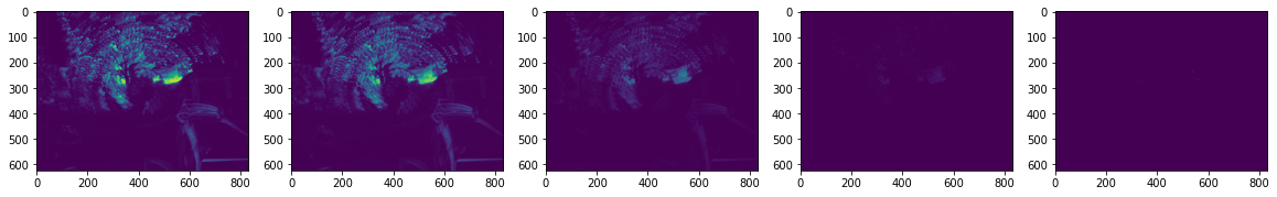
fig, ax = plt.subplots(1,len(detectors))
i=0
for w,d in detectors.items():
    ax[i].imshow((d.variance_background[:,:,1]-init_vars[w][:,:,1])/init_vars[w][:,:,1])
    i+=1
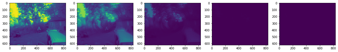
fig, ax = plt.subplots(1,len(detectors))
i=0
for w,d in detectors.items():
    ax[i].imshow((d.average_background[:,:,1]-init_vars[w][:,:,1])/init_vars[w][:,:,1])
    i+=1
The variance field shows an increase in a central circle, which corresponds to the swirl. The variance is higher when object edges are moved as this creates a large observed change, hence the shape of the updated variance.
What is also clear is that the size of the change decreases as the learning rate increases. A too high learning rate means the lesson of motion is not learned.
plt.figure()
for w,c in counts.items():
    plt.plot(c)
plt.legend([str(x) for x in counts], title='Training Weight')
#plt.ylim([0,1])
<matplotlib.legend.Legend at 0x7fab86f3eac8>
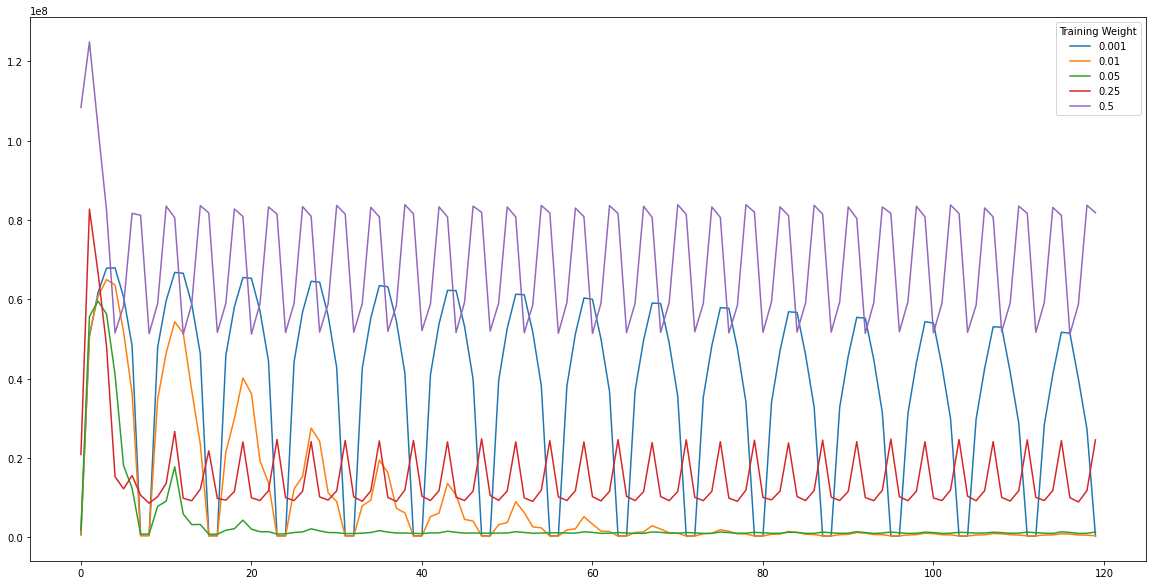
The number of pixels classified as motion tells a similar story, high learning rates adapt to the current frame and do not learn the previous (or noise) leading to a much higher number of detected pixels.
The flip side of this is with low learning rates, which show a long adaption (or no) adaption over time. This can be seen by the recurring peaks in the graph. Ideal learning rates apadt to the background noise at a high rate. The best examples being rates of 0.05 and 0.01 (though to a lesser extent as the learning is sub-optimal).
plt.figure()
for w,c in var.items():
    plt.plot([x/c[0] for x in c])
plt.legend([str(x) for x in counts], title='Training Weight')
<matplotlib.legend.Legend at 0x7fab744e47f0>
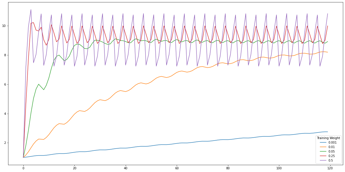
This can again be seen through the mean variance which for this specific synthetic example shows the adaption as the estimated variances converge over time. The low learning rate shows effectively slow adaption while the highest is essentially over fitting through the jagged oscillilations of the curve.
Object on moving background
Now the question is does the adaption of the detectors to a background motion make the detectors insenstive to real “foreground” motion. The truth is nuanced, yes, a region with a shaking tree will have issues detecting a camouflaged person walking in front, however it will have no issues if the person has a blue, red, black t-shirt i.e. a different colour channel as the variance is adapted per channel. The goal of the background learning and detection via variance is to reduce false detections, detecting an object is actually remarkably easy the issue is limmiting to meanigful detections.
#initialsie detectors

weights = [ 0.005,0.01,0.05,0.25]
variance=100
detectors={w:bgd(w,16,example.shape, initial_average=example, initial_variance=variance, minimum_variance=0) for w in weights}
background_counts={}
training_iterations = 10
#train the background
for i in range(training_iterations):
    noisy_image = example + np.random.normal(0, variance**0.5, example.shape)
    # rember the camera clips values
    noisy_image[noisy_image<0]=0
    noisy_image[noisy_image>255]=255
    for w,detector in detectors.items():
        det = detector.apply(noisy_image)
        if background_counts.get(w,None) is None:
            background_counts[w]=np.sum(det)/training_iterations
        else:
            background_counts[w]+=np.sum(det)/training_iterations

init_vars = {w:np.copy(d.variance_background) for w,d in detectors.items()}
Initialised the detectors on a static background, then they should learn the variance of the moving background.
#training against moiving noisy background

counts = {w:[] for w in weights}
var = {w:[] for w in weights}

for cycle in range(12):
    for s in series:
        noisy_image = s + np.random.normal(0, variance**0.5, example.shape)
        noisy_image[noisy_image<0]=0
        noisy_image[noisy_image>255]=255
        for w,detector in detectors.items():
                counts[w].append(np.sum(detector.apply(noisy_image)))
                var[w].append(np.mean(detector.variance_background))

    for s in reversed(series):
        noisy_image = s + np.random.normal(0, variance**0.5, example.shape)
        noisy_image[noisy_image<0]=0
        noisy_image[noisy_image>255]=255
        for w,detector in detectors.items():
                counts[w].append(np.sum(detector.apply(noisy_image)))
                var[w].append(np.mean(detector.variance_background))
This is a huge block of quickly prototyped code. It essentially adds a few practical post processing steps to our detector, such as filtering for a range of object sizes. Also, the number of true and false detections of objects are calculated over the entire run. The code can defintatly be streamlined :)
from skimage.measure import label, regionprops
counts = {w:[] for w in weights}
var = {w:[] for w in weights}
i=0
p=0.25
correct_detections={w:[0] for w in weights}
false_detections={w:[0] for w in weights}

gt=[0]
for cycle in range(10):

    for s in series:
        i+=1
        if np.random.uniform(0,1) < p:
            x= int(400+np.random.uniform(-50,50))
            y= int(200+np.random.uniform(-100,200))
            image = insert_person(s,x,y,value=np.random.uniform(0,255,3).astype(int))
            mask = insert_person(np.zeros(s.shape[0:-1],dtype=bool),x,y,value=1)
            print("person",i)
            gt.append(gt[-1]+1)
        else:
            print("no person",i)
            gt.append(gt[-1])
            mask=np.zeros(s.shape[0:-1],dtype=bool)
            image = np.copy(s)

        noisy_image = image + np.random.normal(0, variance**0.5, example.shape)
        noisy_image[noisy_image<0]=0
        noisy_image[noisy_image>255]=255
        for w,detector in detectors.items():
            dets = detector.apply(noisy_image)
            #plt.figure()
            #plt.imshow(dets)
            objects  = label(dets)
            regions=[]
            for region in regionprops(objects):
                # take regions with large enough areas
                if region.area <= 100 or region.area > 5000:
                    dets[objects==region.label]=0
                else:
                    regions.append(region)
            tp = np.sum(np.logical_and(dets,mask))
            fp = np.sum(np.logical_and(dets,mask==0))
            #print(tp,fp)
            if tp > 1000:
                if gt[-1]!=gt[-2]:
                    correct_detections[w].append(correct_detections[w][-1]+1)
                    false_detections[w].append(false_detections[w][-1]+len(regions)-1)
                else:
                    correct_detections[w].append(correct_detections[w][-1])
                    false_detections[w].append(false_detections[w][-1]+len(regions))

            else:
                correct_detections[w].append(correct_detections[w][-1])
                false_detections[w].append(false_detections[w][-1] + len(regions))

            counts[w].append(np.sum(dets))
            var[w].append(np.mean(detector.variance_background))

    for s in reversed(series):
        i+=1
        if np.random.uniform(0,1) < p:
            x= int(400+np.random.uniform(-50,50))
            y= int(200+np.random.uniform(-100,200))
            image = insert_person(s,x,y,value=np.random.uniform(0,255,3).astype(int))
            mask = insert_person(np.zeros(s.shape[0:-1],dtype=bool),x,y,value=1)
            print("person",i)
            gt.append(gt[-1]+1)
        else:
            print("no person",i)
            gt.append(gt[-1])
            mask=np.zeros(s.shape[0:-1],dtype=bool)
            image = np.copy(s)

        noisy_image = image + np.random.normal(0, variance**0.5, example.shape)
        noisy_image[noisy_image<0]=0
        noisy_image[noisy_image>255]=255
        for w,detector in detectors.items():
            dets = detector.apply(noisy_image)
            #plt.figure()
            #plt.imshow(dets)
            objects  = label(dets)
            regions=[]
            for region in regionprops(objects):
                # take regions with large enough areas
                if region.area <= 100 or region.area > 5000:
                    dets[objects==region.label]=0
                else:
                    regions.append(region)
            tp = np.sum(np.logical_and(dets,mask))
            fp = np.sum(np.logical_and(dets,mask==0))
            #print(tp,fp)
            if tp > 1000:
                if gt[-1]!=gt[-2]:
                    correct_detections[w].append(correct_detections[w][-1]+1)
                    false_detections[w].append(false_detections[w][-1]+len(regions)-1)
                else:
                    correct_detections[w].append(correct_detections[w][-1])
                    false_detections[w].append(false_detections[w][-1]+len(regions))

            else:
                correct_detections[w].append(correct_detections[w][-1])
                false_detections[w].append(false_detections[w][-1] + len(regions))

            counts[w].append(np.sum(dets))
            var[w].append(np.mean(detector.variance_background))
no person 1
no person 2
person 3
no person 4
person 5
no person 6
person 7
no person 8
no person 9
no person 10
person 11
no person 12
person 13
no person 14
person 15
person 16
person 17
person 18
no person 19
person 20
person 21
no person 22
no person 23
no person 24
person 25
no person 26
no person 27
no person 28
no person 29
person 30
no person 31
no person 32
no person 33
no person 34
no person 35
no person 36
no person 37
no person 38
no person 39
no person 40
person 41
person 42
person 43
no person 44
no person 45
no person 46
person 47
no person 48
no person 49
no person 50
person 51
no person 52
person 53
no person 54
no person 55
person 56
no person 57
no person 58
no person 59
person 60
no person 61
no person 62
no person 63
no person 64
person 65
no person 66
person 67
person 68
person 69
person 70
person 71
person 72
no person 73
no person 74
no person 75
no person 76
person 77
person 78
no person 79
person 80
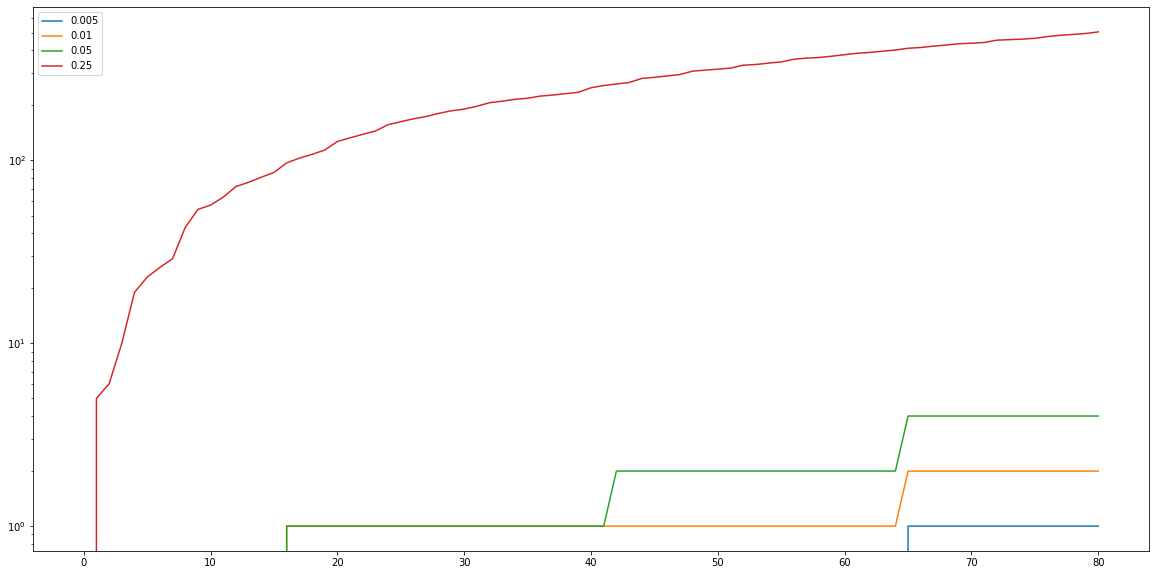
Looking at the number of false detections it is quite clear that the high learning rate has serious issues for this specific test. The lower learning rates have nearly no false detection and are all triggered by the 64 frame in this case.
plt.figure()
fig1 = plt.figure()
ax1 = fig1.add_subplot(111)

for l in list(false_detections.values()):
    ax1.plot(l)
plt.yscale('log')
plt.legend(list(false_detections.keys()))
ax2.set_ylim([1,1e3])
#ax2 = plt.axes([.65, .2, .2, .2])
#for l in list(false_detections.values()):
#    ax2.plot(l)

#ax2.set_xlim([60,70])
#ax2.set_ylim([-1,10])
#plt.setp(ax2, xticks=[], yticks=[])
(1.0, 1000.0)


<Figure size 1440x720 with 0 Axes>
The number of true detections is also important. Here is a plot of the total number of true detections normalised by the ground truth. Again, here we see poor performance from the fast learner.
plt.figure()
for l in list(correct_detections.values()):
    temp = np.array(l)/np.array(gt)
    plt.plot(temp)
#plt.yscale('log')
#plt.ylim([0.75,1.05])
plt.legend(list(correct_detections.keys()))
/home/duncan/.local/lib/python3.7/site-packages/ipykernel_launcher.py:3: RuntimeWarning: invalid value encountered in true_divide
  This is separate from the ipykernel package so we can avoid doing imports until
/home/duncan/.local/lib/python3.7/site-packages/ipykernel_launcher.py:3: RuntimeWarning: invalid value encountered in true_divide
  This is separate from the ipykernel package so we can avoid doing imports until
/home/duncan/.local/lib/python3.7/site-packages/ipykernel_launcher.py:3: RuntimeWarning: invalid value encountered in true_divide
  This is separate from the ipykernel package so we can avoid doing imports until
/home/duncan/.local/lib/python3.7/site-packages/ipykernel_launcher.py:3: RuntimeWarning: invalid value encountered in true_divide
  This is separate from the ipykernel package so we can avoid doing imports until


<matplotlib.legend.Legend at 0x7fab870077b8>
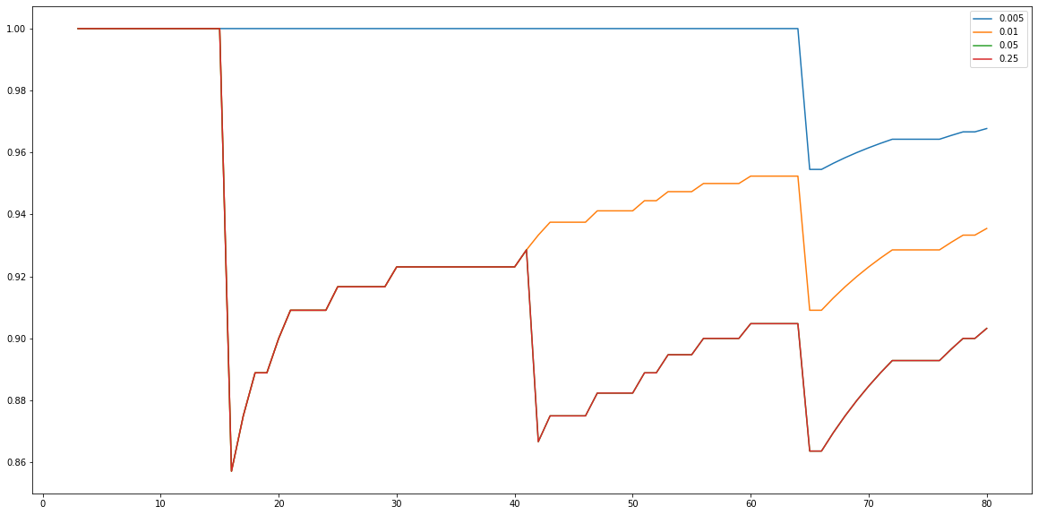
This notebook is by no means a defintiative analysis of this motion detecting class, however it shows the pitfalls of some paramters. The high learning rates could probably have imporved performance if a minimum variance is used. The size filtering in the example above is also another aspect which can help improve the detection. However, this does demonstrate that this alogrithm is quite robusrt, detecting >90% of motion events on a highly deformed background.